Gene level evaluation

In this notebook we focus on how to train InterScale using the molecular cartography dataset used from Legnini et al., 2023 which we preprocessed in the previous tutorial.

Requirements:

• inference results in the anndata object

• trained model to load inference results

Import packages

import scanpy as sc
import numpy as np
import matplotlib.pyplot as plt
import seaborn as sns
from pathlib import Path
import os

import warnings

# gene program import
import gseapy as gp
import matplotlib as mpl
import pandas as pd

warnings.filterwarnings("ignore")

import interscale
from interscale.config import load_config
from interscale.evaluation import (
    gene_loadings,
    calculate_gene_ranks,
    latent_rank_report,
    get_genes_dim,
    calculate_dim_importance,
)

interscale.tl.set_full_reproducibility()

import sys

# Find repo root by locating paths.py
BASE_DIR_PROJECT = Path.cwd().resolve().parent.parent

sys.path.insert(0, str(BASE_DIR_PROJECT))
DATA = "legnini"
RESULTS_DIR = Path(f"{BASE_DIR_PROJECT}/results/{DATA}")

Load data and model

To load the model, check in the previous tutorial 1_model_training.ipynb in the model training for the path where the model was saved to.

adata = sc.read_h5ad(f"{BASE_DIR_PROJECT}/data/{DATA}_trained.h5ad")
cfg = load_config(Path(f"{BASE_DIR_PROJECT}/config_files/{DATA}_example.yaml"))

interscale.model.CombinedModel._setup_anndata(
    adata=adata,
    prediction_task=cfg.dataset.prediction_task,
    layer_key=cfg.dataset.layer_key,
    sample_key_list=cfg.dataset.sample_key,
    prediction_obs=cfg.dataset.prediction_obs,
    view_registry=False,
)

dual_combined_model = interscale.model.CombinedModel.load(
    os.path.join(RESULTS_DIR),
    adata,
    cfg,
    local_component=True,
    global_component=True,
)

Loading model from /Users/francesca.drummer/Documents/1_Projects/A3-InterScale/interscale/results/legnini/dual_legnini23_regr_node_44_GCN_self-attn-transformer_model.pt
Unclear checkpoint format. Attempting remapping anyway.
State dict remapping applied. Source detected: unknown

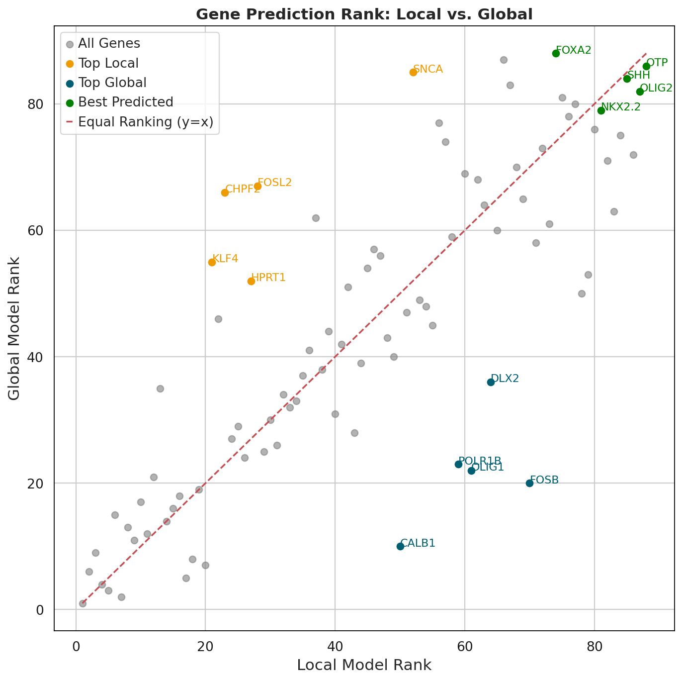
Gene rank analysis

First we check whether the local and global embeddings capture different genes and which genes are better learned by the local vs global component.

For each gene, we computed: Local Rank: Ranking based on local model reconstruction performance XL Global Rank: Ranking based on global model reconstruction performance XG Rank Difference: Local Rank - Global Rank, indicating model preference Average Rank: (Local Rank + Global Rank) / 2, representing overall predictive quality

df = calculate_gene_ranks(adata, layers_local_pred="_y_pred_local", layers_global_pred="_y_pred_global")

interscale.pl.gene_ranks(df, top_n=5)

Gene loadings

standardize gene loadings meaning = change in gene g (in gene SD units) per 1 SD increase in latent dimension k.

gene_loadings(
    adata,
    dual_combined_model,
    local_latent_key="_global_emb",
    global_latent_key="_global_emb",
    layer_key="log1p_norm",
)

AnnData object with n_obs × n_vars = 43762 × 88
    obs: 'Cell', 'Area', 'x', 'y', 'sample', 'condition', 'organoid', 'obs_names', 'split', '_scvi_sample_key_0', '_scvi_split_key', '_cls_horizontal', '_cls_vertical'
    var: 'gene_ids', 'feature_types'
    uns: '_scvi_manager_uuid', '_scvi_uuid', 'spatial_neighbors'
    obsm: '_attn_matrix', '_global_emb', '_local_emb', 'spatial'
    varm: '_local_std_gene_loadings', '_global_std_gene_loadings'
    layers: '_y_pred_global', '_y_pred_local', 'log1p_norm', 'norm_ftsqrt', 'raw'
    obsp: 'spatial_connectivities', 'spatial_distances'

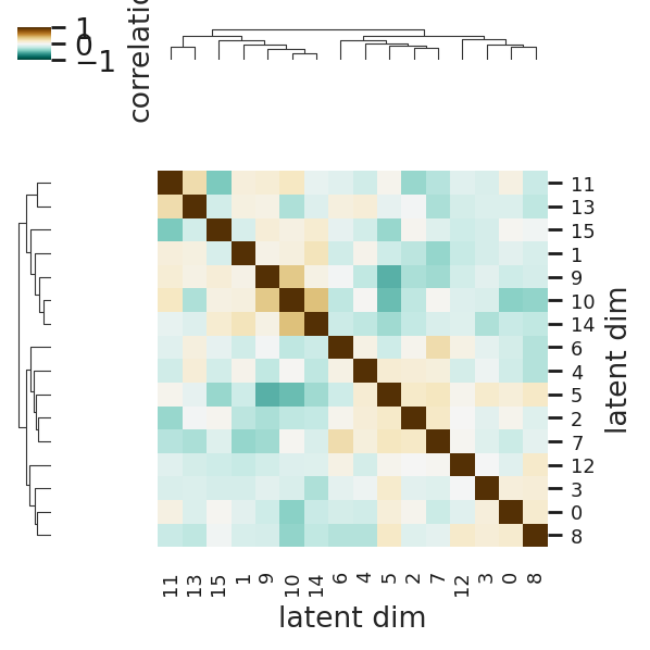
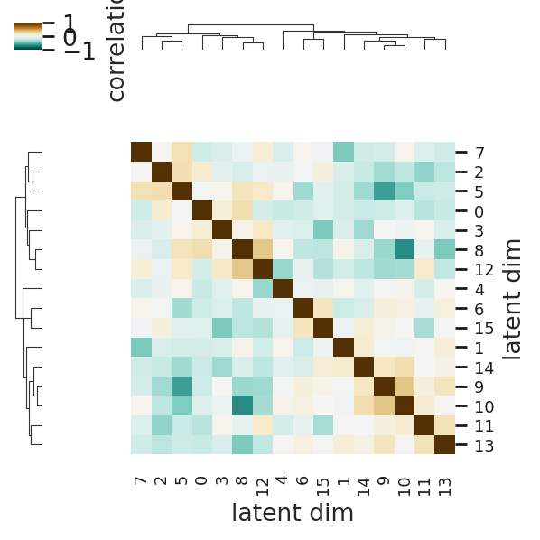
First we check the correlation between each embedding dimension. If the matrix is almost diagonal, we can assume linea independence.

# Check rank:
rep_global = latent_rank_report(adata, z_key="_global_emb")
rep_local = latent_rank_report(adata, z_key="_local_emb")
print(rep_global)
print(rep_local)

{'z_key': '_global_emb', 'n_obs': 43743, 'n_dims': 16, 'rank': 16, 'linearly_independent': True}
{'z_key': '_local_emb', 'n_obs': 43762, 'n_dims': 16, 'rank': 16, 'linearly_independent': True}

interscale.pl.latent_correlation(
    adata, z_key="_local_emb", vmax=1.0, cmap="BrBG_r", title="Local Embedding", figsize=(4, 4)
)
interscale.pl.latent_correlation(
    adata, z_key="_global_emb", vmax=1.0, cmap="BrBG_r", title="Global Embedding", figsize=(4, 4)
)

<seaborn.matrix.ClusterGrid at 0x3a1640510>

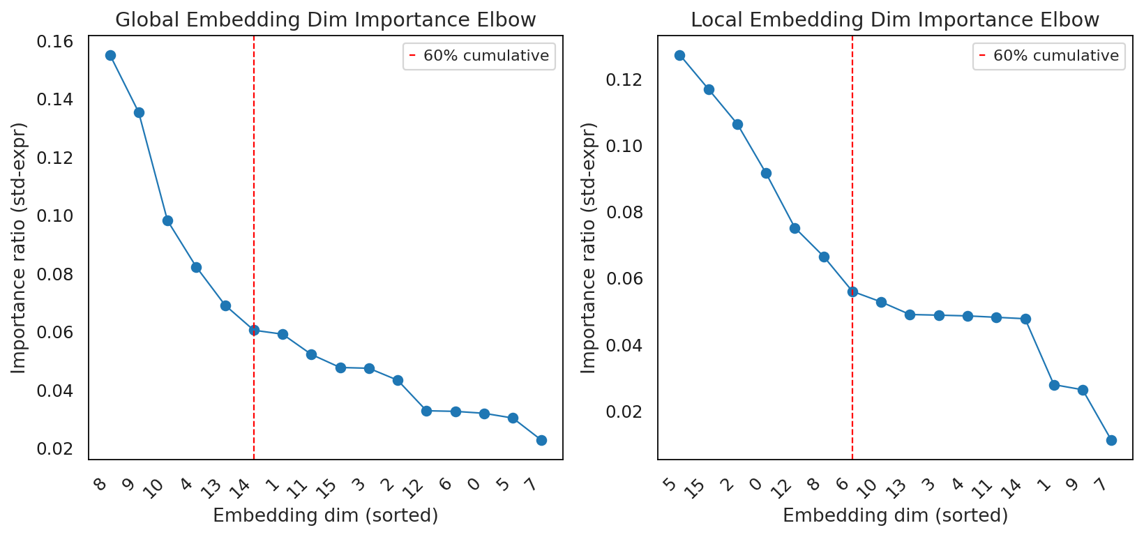
result_global = calculate_dim_importance(
    adata,
    s_key="_global_std_gene_loadings",
    z_key="_global_emb",
    mode="full",
    use_ratio=True,
    cumulative_cutoff=0.60,
    spacing=2,
)
result_local = calculate_dim_importance(
    adata,
    s_key="_local_std_gene_loadings",
    z_key="_local_emb",
    mode="full",
    use_ratio=True,
    cumulative_cutoff=0.60,
    spacing=2,
)

fig, axes = plt.subplots(1, 2, figsize=(12, 5))
interscale.pl.dim_importance_elbow(result_local, title="Local Embedding Dim Importance Elbow", ax=axes[1])
interscale.pl.dim_importance_elbow(result_global, title="Global Embedding Dim Importance Elbow", ax=axes[0])

60% cumulative variance reached with 7 dimensions:
Embedding dimensions (sorted by importance):
[5, 15, 2, 0, 12, 8, 6]

60% cumulative variance reached with 6 dimensions:
Embedding dimensions (sorted by importance):
[8, 9, 10, 4, 13, 14]

<Axes: title={'center': 'Global Embedding Dim Importance Elbow'}, xlabel='Embedding dim (sorted)', ylabel='Importance ratio (std-expr)'>

Expression Filtering

Argument	Effect
min_frac	Remove rare genes
min_sd	Remove low-variance genes

Scoring Choices

Argument	Meaning
rank_by=”loading”	Pure decoder sensitivity
rank_by=”loading_x_sd”	Favor highly variable genes
residualize=True	Use only unique component of dimension

Specificity Control

Argument	Meaning
enforce_specificity	Force genes to be dimension-specific
specificity_mode=”ratio”	max/second criterion
specificity_min	How strict the specificity must be

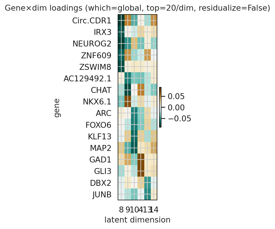
gene_by_dim_heatmap interpretation:

So:

• Dark brown → strong positive association with that dimension

• Dark green → strong negative association

• Near white → little association

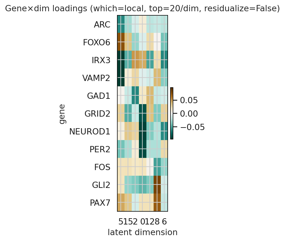
Select the local and global dimensions.

global_dim = [8, 9, 10, 4, 13, 14]
local_dim = [5, 15, 2, 0, 12, 8, 6]

df_global, ax = get_genes_dim(
    adata,
    which="global",
    dims=global_dim,
    n_top=20,
    X_layer="log1p_norm",
    min_frac=0.1,
    rank_by="loading_x_sd",
    enforce_specificity=True,
    specificity_min=1.5,
    # residualize=True,
    plot=True,
    figsize=(3.3, 5),
)

df_local, ax = get_genes_dim(
    adata,
    which="local",
    dims=local_dim,
    n_top=20,
    X_layer="log1p_norm",
    min_frac=0.1,
    enforce_specificity=True,
    rank_by="loading_x_sd",
    specificity_min=1.5,
    # residualize=True,
    plot=True,
    figsize=(3.3, 5),
)

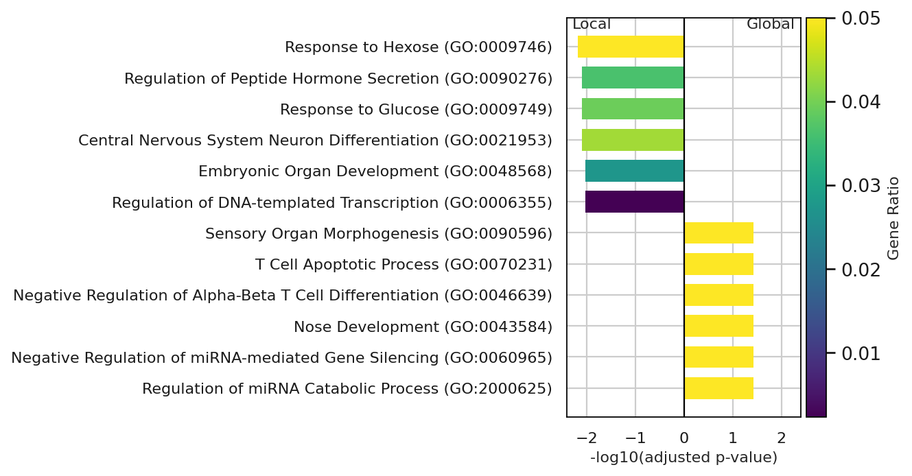
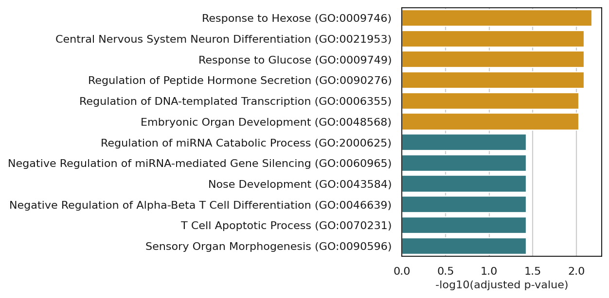
Identify gene programs

In the next step, we take those top genes associated with the local and global latent dimensions and ask whether they form coherent biological programs.

global_genes = df_global.index
local_genes = df_local.index

shared = global_genes.intersection(local_genes)
unique_local = local_genes.difference(global_genes)
unique_global = global_genes.difference(local_genes)

print("Shared:", shared.tolist())
print("Unique local:", unique_local.tolist())
print("Unique global:", unique_global.tolist())

Shared: ['IRX3', 'ARC', 'FOXO6', 'GAD1']
Unique local: ['FOS', 'GLI2', 'GRID2', 'NEUROD1', 'PAX7', 'PER2', 'VAMP2']
Unique global: ['AC129492.1', 'CHAT', 'Circ.CDR1', 'DBX2', 'GLI3', 'JUNB', 'KLF13', 'MAP2', 'NEUROG2', 'NKX6.1', 'ZNF609', 'ZSWIM8']

enr_global = gp.enrichr(
    gene_list=unique_global.tolist(),
    gene_sets="GO_Biological_Process_2025",
    organism="human",  # or "Mouse"
    outdir=None,
)
enr_global.results.head()

	Gene_set	Term	Overlap	P-value	Adjusted P-value	Old P-value	Old Adjusted P-value	Odds Ratio	Combined Score	Genes
0	GO_Biological_Process_2025	Regulation of miRNA Catabolic Process (GO:2000...	1/5	0.002997	0.037343	0	0	454.181818	2638.914119	ZSWIM8
1	GO_Biological_Process_2025	Negative Regulation of miRNA-mediated Gene Sil...	1/6	0.003595	0.037343	0	0	363.327273	2044.882815	ZSWIM8
2	GO_Biological_Process_2025	Nose Development (GO:0043584)	1/7	0.004193	0.037343	0	0	302.757576	1657.396457	GLI3
3	GO_Biological_Process_2025	Negative Regulation of Alpha-Beta T Cell Diffe...	1/8	0.004791	0.037343	0	0	259.493506	1385.975083	GLI3
4	GO_Biological_Process_2025	T Cell Apoptotic Process (GO:0070231)	1/8	0.004791	0.037343	0	0	259.493506	1385.975083	GLI3

enr_local = gp.enrichr(
    gene_list=unique_local.tolist(),
    gene_sets="GO_Biological_Process_2025",
    organism="human",  # or "Mouse"
    outdir=None,
)
enr_local.results.head()

	Gene_set	Term	Overlap	P-value	Adjusted P-value	Old P-value	Old Adjusted P-value	Odds Ratio	Combined Score	Genes
0	GO_Biological_Process_2025	Response to Hexose (GO:0009746)	2/25	0.000031	0.006590	0	0	347.304348	3601.323532	NEUROD1;VAMP2
1	GO_Biological_Process_2025	Central Nervous System Neuron Differentiation ...	2/46	0.000108	0.008114	0	0	181.354545	1656.578768	NEUROD1;GRID2
2	GO_Biological_Process_2025	Response to Glucose (GO:0009749)	2/51	0.000133	0.008114	0	0	162.808163	1453.350008	NEUROD1;VAMP2
3	GO_Biological_Process_2025	Regulation of Peptide Hormone Secretion (GO:00...	2/55	0.000155	0.008114	0	0	150.490566	1320.548882	NEUROD1;PER2
4	GO_Biological_Process_2025	Regulation of DNA-templated Transcription (GO:...	5/2139	0.000243	0.009293	0	0	20.921978	174.126969	NEUROD1;PER2;PAX7;FOS;GLI2

df_local = enr_local.results
df_global = enr_global.results

df_local["group"] = "Local"
df_global["group"] = "Global"

combined = pd.concat(
    [df_local.sort_values("Adjusted P-value").head(6), df_global.sort_values("Adjusted P-value").head(6)]
)

combined["-log10(padj)"] = -np.log10(combined["Adjusted P-value"])

combined = combined.sort_values("-log10(padj)", ascending=False)

palette = {"Global": "#27828E", "Local": "#EE9B00"}

plt.figure(figsize=(8, 4))

sns.barplot(data=combined, y="Term", x="-log10(padj)", hue="group", palette=palette, legend=False)

plt.xlabel("-log10(adjusted p-value)", fontsize=10)
plt.ylabel("", fontsize=10)
# plt.title("GO enrichment: global vs local embeddings", fontsize=10)

plt.xticks(fontsize=10)
plt.yticks(fontsize=10)

# plt.legend(title="", fontsize=10)

plt.tight_layout()
# plt.savefig("figures/gene_programs.png", dpi=300, bbox_inches="tight")
plt.show()

# --- Prepare dataframe ---
plot_df = combined.copy().reset_index(drop=True)

# --- Compute Gene Ratio ---
plot_df["gene_ratio"] = plot_df["Overlap"].str.split("/").apply(lambda x: int(x[0]) / int(x[1]))

# --- Clip extreme values (stabilize color contrast) ---
clip_max = 0.05  # adjust if needed
plot_df["gene_ratio_plot"] = plot_df["gene_ratio"].clip(upper=clip_max)

# --- Signed values for diverging bars ---
plot_df["signed_log10"] = plot_df["-log10(padj)"]
plot_df.loc[plot_df["group"] == "Local", "signed_log10"] *= -1

# --- Sort by absolute significance ---
plot_df = plot_df.sort_values(by="signed_log10", key=lambda s: s.abs(), ascending=True).reset_index(drop=True)

# --- Colormap setup ---
cmap = plt.cm.viridis
norm = mpl.colors.Normalize(vmin=plot_df["gene_ratio_plot"].min(), vmax=plot_df["gene_ratio_plot"].max())

# --- Create figure ---
fig, ax = plt.subplots(figsize=(8, 4.5))

# --- Plot bars ---
ax.barh(
    y=plot_df["Term"],
    width=plot_df["signed_log10"],
    color=cmap(norm(plot_df["gene_ratio_plot"])),
    edgecolor="none",
    height=0.7,
)

# --- Center line ---
ax.axvline(0, color="black", linewidth=1)

# --- Symmetric x-limits ---
max_val = plot_df["-log10(padj)"].max()
ax.set_xlim(-max_val * 1.1, max_val * 1.1)

# --- Labels ---
ax.set_xlabel("-log10(adjusted p-value)", fontsize=10)
ax.set_ylabel("")
ax.tick_params(axis="x", labelsize=10)
ax.tick_params(axis="y", labelsize=10)

# --- Optional group labels ---
ax.text(-max_val * 1.05, len(plot_df) - 0.5, "Local", ha="left", va="bottom", fontsize=10)
ax.text(max_val * 1.05, len(plot_df) - 0.5, "Global", ha="right", va="bottom", fontsize=10)

# --- Colorbar ---
sm = mpl.cm.ScalarMappable(cmap=cmap, norm=norm)
sm.set_array([])
cbar = fig.colorbar(sm, ax=ax, pad=0.02)
cbar.set_label("Gene Ratio", fontsize=10)

# --- Layout & save ---
plt.tight_layout()
plt.savefig("../../../figures/gene_programs_diverging_gene_ratio.png", dpi=300, bbox_inches="tight")
plt.show()